TDS Spectrum Viewer
Ver.0.3
- About this software
This software is the spectrum viewer and analyzer for terahertz time-domain spectroscopy.
This software is free software program. Download, professional use, re-distribution of this software is free, but copyrighted by H. Hoshina.
- Introduction
- You can see your spectrum immediately after the measurement without any commercial graph software. (You do not need to pay a lot for Origin or Igor)
- You can handle a lot of data by tree view, which may reduce confusion.
- You can directly print out your data via software.
- Input format
THz-TDS time-domain waveform (CSV text)
Fourier Transformed Spectrum (CSV text) - Output format
THz-TDS time-domain waveform (CSV text)
Fourier Transformed Spectrum (CSV text)
Absorbance (CSV text)
Refractive index (CSV text)
- The project can be saved by a binary data.
- Datas are displayed in a tree view
- Fourier Transform(FFT)
Input time range and output frequency range can be set.
You can choose Zero-Filling points and apodization function. - Absorbance
Absorbance or transmittance can be selected for output.
You can output absorbance based on Log10 or Loge. - Refractive index is calculated by using initial value of n and k, and sample thickness.
- You can change the view of all graphs by mouse and keyboard
expand
reduction
offset
previous view
graph color change
read axis value
- You can copy data and image to the clipboard.
You can paste data to Origin
- You can print out your graph with legends
- System requirements
WindowsXP or later
.NET Framework 2.0 or later
- Download
TDS Spectrum Viewer 0.3.3 (361kB)
- Install
Unzip the downloaded file and run setup.
If .NET Framework is not installed, the installer will automatically download and install that.
- Functions
- Input file format
- Terahertz time domain wavefoams
Software read text files saved by THz-TDS.
Comments in the first lines of the file are allowed (i.e. measurement conditions).
If the first character of the line is special character ("#" as a default. Changeable in the settings menu.),the line will be ignored.
Also, the comment will be recorded in the "info" text. (You can see "info" by right clicking the data)
The first column is treated as time, the second column is as a signal intensity. (Changeable in settings menu)
Columns should be separated by ",", space or tab.
Datas should be more than 50 lines.
The unit of time is ps (default). You can change unit to fs or stage position (mm or microns, single path or double path) in the settings menu.
The time data will be saved as ps.
The signal must be sampled in same interval. (The time of each data are not directly taken from the data, but calculated by dividing the distance between first data and last data by the data number)
example
#2009/07/14 23:18
#measurement mode=transmission
#start point=0[μm]
#resolution=1.929050 [cm-1]
#A/Dconversion=0.3164[μm]
#repetition time=1
#Data aquisition interval=0[ms]
#Scan time=20
#Data points=4096[pts.]
#Upper limit of frequency=3950.695322[cm-1]
#Pressure=6.9[Pa]
#Stage velocity=800[μm/sec]
0.000000 -0.010986
0.004219 -0.005798
0.008437 -0.001831
0.012656 -0.009460
0.016875 0.006409
0.021093 -0.001831
0.025312 -0.012817
0.029531 -0.015564
0.033749 -0.010681
0.037968 -0.008850
.
.
.
- FT Data
Read text file of Fourier Transformed data.
Comments in the first lines of the file are allowed (i.e. measurement conditions).
If the first character of the line is special character ("#" as a default. Changeable in the settings menu.),the line will be ignored.
Also, the comment will be recorded in the "info" text. (You can see "info" by right clicking the data)
The first column is treated as frequency, the second column as a power, and the third column as phase. (Changeable in settings menu)
Columns should be separated by ",", space or tab.
Datas should be more than 50 lines.
- Terahertz time domain wavefoams
- Data load
- Drug & Drop
Drug & Drop file(s) on the program window
When the file(s) is dropped on the area (1), it will be treated as a time domain waveform.
When the file(s) is dropped on the area (2), it will be treated as the same format as is displayed.
- File dialog
Choose "Open Time Domain" or "Open FT Data" menu in the Button or File menu.
- Options when multiple files are read (available for time domain data)
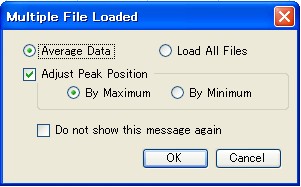
"Average Data" average the intensities of all files and load
"Load all Files" load all files separately
"Adjust peak position" adjust time of peak maximum when multiple files are averaged. This option will be useful when your system has jitter.
"Do not show this message again" checkbox enables you to skip this menu. You can see this menu again in the settings menu.
- Drug & Drop
- Graph manipulation
The datas will be displayed on the different graph windows depending on its type.
The graph window can be switched by tab.
- Time Domain: Time domain waveform
- Single Beam: Power spectrum obtained by FFT. (Log scale)
- Phase: Phase spectrum obtained by FFT
- Absorbance: Absorbance spectrum calculated by dividing two power spectra. You can select ether absorbance or transmittance by settings menu.
- n: Real part of refractive index
- k: Imaginary part of refractive index
Graph drawing has two options, "Quick mode" and "normal mode". "Quick mode" skips data according to the display resolution. (same as "speed mode" in Origin)
Sometimes, details of the waveform may not be shown correctly in "Quick mode". In such case, please uncheck this option. (drawing may become slower)
Graph view can be manipulated by the buttons or right-click menu, as follows
- Expand, Reduction
- Click ZoomIn, or ZoomOut buttons, or use right-click menu. Select area by mouse.
- Mouse scroll change expand the area, centered the cursor position
- Directly put values of the axis
- Shift displayed area
- Click "Move Axis" button or right click menu, and drug on the graph
- "Up", "Down", "Right", "Left" key on the keyboard
- Back to previous view
- Click "Previous scale" button or right click menu. The displayed area goes back to previous.
- Show all
- Click "ShowAll" button or right click menu. All data range will be displayed.
- Only when the "transmittance" is shown, the Y axis is set to 0 to 100.
- Read Cursor Position
- Click "ReadCursorPosition" button and click graph. The cursor position will be displaced on the status bar.
- Click "ReadDataPosition" button and click graph. the nearest
data value will be shown in the status bar.
The cursor can move by "right" and "left" key.
The value will be taken from that selected in the tree view.
- Offset
Graphs are offset. The values of the data itself does not change.- Click "OffsetWave" and drug. The selected plot shift to Y direction.
- ResetOffset button makes the all offset value as 0.
- The +Offset, -Offset buttons set equal offset for all plots.
- Click "OffsetWave" and drug. The selected plot shift to Y direction.
- Datas on the tree view
Loaded datas are shown in the tree view.
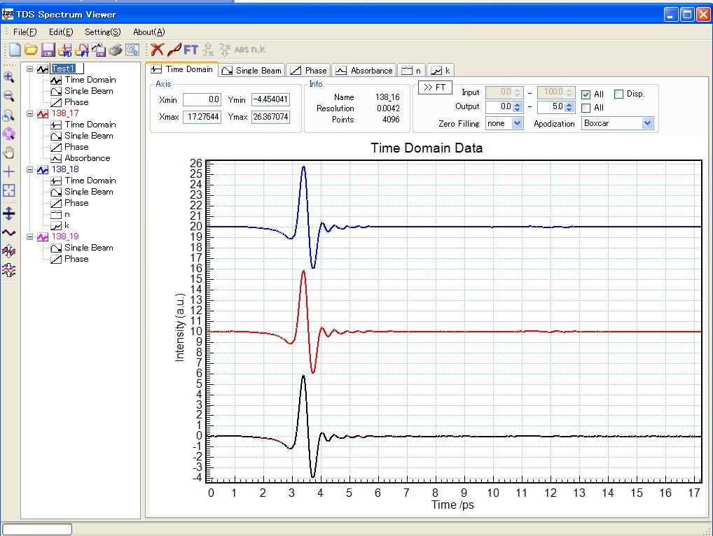
Each data has parent node which contains time domain, FT, absorbance, n and k.
The name of the parent node can be changed.
When the parent node is right-clicked, following menu will be shown- plot color changed
- delete data
Right click of child menu shows- plot color change
- delete data
- Show or not show the plot
- Save data
- Copy data to the clipboard (CSV, can be paste on Origin)
- show information of the data
- Fourier transform
Fourier transform of the time domain data (FFT) is calculated based of the algorithm of Numerical Recipes.
The selected time domain data will be Fourier transformed by clicking FT tool button or FT button on the time-domain graph window.
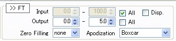
You can set options as follows- Input range
This option set the input time range of FFT.
When "All" checkbox is checked, all of the time domain data will be used for FFT.
When "All" checkbox is not checked, time domain data in the input time range will be used for FFT.
When "Disp" checkbox is checked, the displayed time range will be Fourier transformed.
If the number of data points is not 2^n, 0 value will be add to the end. (for example, time domain data of 5000 pts will be extended to 8192 pts by adding 0) - Output range
This option set the output frequency range of FFT.
When "All" checkbox is checked, all frequency range of the FFT will be output. - ZeroFilling
This option set the zero-filling factor.
The input data will be increased by adding 0, which makes the frequency resolution better. - Apodization
Multiplied apodization function to the time domain data.- Boxcar:1
- Cosine:[0.5*{1+cos(PI*x/xmax)}]^2
- Triangle:1-x/xmax
- Blackman:0.42+0.50*cos(PI*x/xmax)-0.08*cos(2PI*x/xmax)
- Blackman-Harris:0.42323+0.49755*cos(PI*x/xmax)-0.07922*cos(2PI*x/xmax)
- Happ-Genzel: 0.54+0.46*cos(PI*x/xmax)
- Hanning:0.5*{1+cos(PI*x/xmax)}
The options of FFT will be recorded in the "info" in each data nodes.
- Input range
- Absorbance
Absorbance or Transmittance (you can change in the settings menu) is calculated by clicking "Abs" button.
The reference of the Single Beam spectrum should be selected in the pull-down menu.
The sample and reference data must contain same data points.
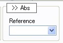
Absorbance is calculated based on the following equation
-Log(SBSsample/SBSreference)
You can use Log10 or Loge in the Settings menu.
The calculation history will be recorded in the "info" in the data nodes.
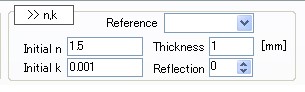
- Refractive indexes
The calculation of the refractive index is based on the method in "M.Hangyo.et al. Meas.Sci.Technol. 13 (2002) pp.1727-1738"
You should set thickness of the sample, initial values of n and k.
- Data improvement
- Delete peaks in Time-Domain Data
Click "Delete peaks" button and select time window to delete peaks in the time domain data.
This option is useful to remove multi-reflection, and smooth spectra.
- Shift Phase for 2PI
Click "Phase Shift" button for shift phase for 2PI.
- Delete peaks in Time-Domain Data
- Save or load data and project
- The data on the tree view can be saved as a text (CSV) file.
The 1st column is time (frequency), and the 2nd column is the intensity, separated by the character "," (Can be changed in the Settings menu)
The "info" can be saved as header of the saved file.
- The project can be saved.
Default file extension is "TDS".
- The data on the tree view can be saved as a text (CSV) file.
- Copy to the clipboard
- Data or graph can be copied to the clipboard
- Graph is copied as a bitmap image
- Data or graph can be copied to the clipboard
- Print
Graphs can be printed out
The name of the data node can be printed out as a legend.
- Input file format